Consistency analysis of lidar survey data
INCOMPLETE
DRAFT, 19 MARCH 2007
Ralph A. Haugerud
U.S. Geological Survey
Seattle, WA
rhaugerud@usgs.gov
Extensive swath overlap in most lidar (also known as airborne laser
swath mapping, or ALSM) surveys makes it possible to generate robust
estimates of the internal reproducibility of a lidar survey--that is,
how consistent it is. In the course of such consistency analysis it is
convenient to also measure how complete a survey is. Such measures of
reproducibility and completeness are powerful, inexpensive tools for
evaluating the quality of lidar data and should underlie many of the
technical specifications in contracts for the collection of lidar
survey data.
This document explores the rationales and approximations that underlie
consistency analysis and explains the format in which the CONSISTENCY
code (Haugerud, in preparation) reports the results of such analyses.
CONSISTENCY builds on 7 years experience contracting for and
evaluating lidar survey data collected by several vendors in the
Pacific Northwest and elsewhere, primarily with the Puget Sound Lidar Consortium
(PSLC) (e.g., Haugerud and others, 2003).
Table of Contents
What is missing?
Voids must be found by inspection
Accuracy of return classification is unquantified
Little leverage on range calibration
Careful survey design can make long-period errors invisible
Spatial correlation of error is not quantified
Users' tolerances for error at different wavelengths have not been
explored
An error model for
lidar DEMs
Lidar DEMs (digital elevation models) are made by a three step process.
- Measure, with a lidar
survey, the positions of points in the target region
- Classify some measured
points as ground
- Interpolate classified
ground points to a continuous bare-earth model
We can thus approximate the error of a lidar DEM as
( measurement_error2 + classification_error2 + interpolation_error2 ) 1/2
This error equation is only approximate as measurement, classification,
and interpolation steps are not entirely independent. Large measurement
errors, if
they have little spatial correlation, increase the likelihood of
classification errors. Classification errors can be reduced by
being more conservative in identifying points as ground ("if in doubt,
throw it out"), but at the cost of increasing
interpolation error.
Several important points follow from this simple analysis.
- The errors that matter to users of lidar elevation models will be
larger than the measurement errors commonly quoted by lidar data
providers.
- In terrain where classification errors are significant--consider
the case where 1 nominal ground point in 100 is actually a point on a
tree 10 meters above the surrounding landscape--even a small proportion
of misclassified points can be a significant source of DEM error. A
requirement that 90%, 95%, or 97% of not-ground points be identified as
such does little to guarantee a useful ground model.
- The magnitude of interpolation error depends on both ground-point
spacing and the local curvature of the ground surface. Landscapes with
extensive diffusional smoothing require fewer ground points per unit
area to achieve a given DEM accuracy than landscapes with abundant
sharp slope breaks.
- In densely forested landscapes, interception of most laser pulses
by the forest canopy results in a small fraction--commonly 1/3 or
less--of
laser pulses producing ground returns. Such sparse ground returns
increase interpolation error. Classification of returns as ground is
easier with denser lidar data that provide a more complete
picture of the target region. For these reasons, more accurate DEMs of
forested terrain may be most readily obtained by a densifying the
survey, not increasing its accuracy.
- In smooth landscapes, lidar surveys may oversample the landscape
and interpolation from ground points to a surface model with a
smoothing function that does not pass through every ground point, such
as Mitasova and ___'s regularized spline with tension (_ref_), may
reduce the error of the DEM by averaging out some pulse-to-pulse lidar
measurement error ("laser
noise"). In angular landscapes, or forested landscapes where the ground
is sparsely sampled because the canopy intercepts all of most laser
pulses, a
lidar survey may undersample the landscape and interpolation with a
smoothing function is likely to increase DEM error.
If we compare 1st-return surfaces from overlapping swaths of lidar data
and minimize interpolation error by restricting the analysis to areas
with little or no curvature, we readily quantify much of the
measurement error in a lidar survey. If we compare surfaces
interpolated from classified ground points from overlapping swaths, we
quantify the sum of classification error, interpolation error, and much
(not all) of the measurement error, but we overestimate interpolation
error because each single-swath surface is built from sparser ground
points than the aggregate (multi-swath) survey and thus has greater
interpolation error.
A user's model of
lidar measurement errors
not yet written
Completeness
not yet written
Reading the
CONSISTENCY report
CONSISTENCY generates a linked set of HTML pages (text and images) that
quantitatively describe a lidar data set, facilitate visual evaluation
of certain unquantifiable aspects, and facilitate exploration of the
nature and causes of measurement and DEM errors. It is designed as a
tool for routine quality assessment and as means for purchaser and
vendor to communicate about data quality issues. This section
describes and explains the elements of a CONSISTENCY report.
Graphic index to
analyzed tiles
Estimages of global accuracy and
completeness
Exclusion
of tiles
Accuracy and completeness estimates (below)
may be severely compromised by large areas of open water that may not
produce lidar returns unless at nadir (specular reflection sends
all laser light somewhere other than the sensor) and that may change
elevation between successive swaths because of time-varying river
discharge,
the tide, winds, or drying of fields. For this reason, the analyst may
choose to
exclude some tiles from the calculation of all-survey averages.
Similarly, a tile of data
may be excluded if it captures large changes between swaths due to
construction or vehicle movement.
P1 &
P2 P1
and P2 are best estimates of the accuracy of location of individual
lidar return points. P1 is an
estimate of the root mean square (RMS) Z
reproducibility of repeated point
measurements. P2 is an estimate of the root
mean square XY reproducibility of repeated measurements. If a surface
is interpolated from these returns with an interpolator
that honors all return points, P1 is an estimate of RMS Z
measurement error of this surface
on flat ground and P2 describes how likely the Z measurement error of
this surface is to increase
as local slope increases.
P1 and P2 are
calculated as:
- Take the complete set of difference - curvature - slope (DCS)
triplets from swath overlaps in the analyzed tiles, including multiple
DCS
triplets where more than two swaths cross.
- Extract the difference - slope (DS) slice for curvature
< 5
- Filtering by local curvature is not sufficient to identify all
cases where swath surfaces differ because one swath has penetrated into
(or through) forest canopy and the overlapping swath does not. To
further eliminate such cases, which skew the distribution
of differences to high values, truncate by eliminating all cases where
difference is greater than the larger of 100 cm or 3 * RMS difference
of the complete DS (C<5) data set
- Calculate least-squares best-fit quadratic to remaining DS values
- P1 = y-intercept (Z difference at local slope = 0)
- P2 = (Z difference at local slope = 100)2 - P12)
1/2 / (average value of sin(theta), theta = 0 to
360)
- DCS triplets are extracted from rasters with cellsize ~ 50% of
nominal ground-return spacing. Thus the apparent sample size is ~4
times the number of lidar returns that contribute to the calculation.
The n reported for
the P1 - P2 calculation is the number of DS couplets divided by 4
The values of P1 and P2 are linked to graphs of difference versus
slope, difference versus curvature, and curvature versus slope.
1st-return surface RMS Z
reproducibility
One can calculate the global reproducibilty of lidar survey
measurements as the RMS difference between interpolated
1st-return surfaces for overlapping swaths, with no compensation or
masking to exclude the effects of local slope. The calculated accuracy
is that of a surface where XY error independent of Z error has no
meaning, as any XY error is translated into Z error. For a
constant measurement accuracy, RMS Z reproducibility values are greater
in areas with greater average slopes.
For this calculation, CONSISTENCY minimizes interpolation errors due
large local
curvatures by (1) identifying raster cells where local curvature
exceeds a test value, (2) buffering out a predetermined number of cells
from large-curvature cells, and (3) excluding large-curvature cells and
the buffered region from calculation of RMS differences. This exclusion
is pictured in the 1st-return swath difference images, where
unsaturated
colors mark the excluded areas and saturated colors mark the areas for
which differences are averaged. Where more than two swaths overlap,
multiple differences can be
calculated, but only one, the difference between the oldest and
youngest swath, is used for calculation of the per-tile
1st-return reproducibility.
Interpolation error is further minimized (and calculation of data set
completeness facilitated) by aggressive masking of NODATA areas. For
single-swath surface rasters, any cells that are more than a predefined
distance (typically 1.5 - 2 times the nominal ground spacing of laser
pulses) are tagged as NODATA.
RMS reproducibility is calculated for each tile, as is the 95th
percentile confidence limit (that is, the value which is exceeded by
only 5% of the observed differences. For a normal distribution, the
95th percentile confidence limit is approximately 1.96 * RMS
difference. Observed differences within most lidar data sets conform to
this relationship. A few don't, indicating that for these data sets the
error distribution is not Gaussian.
Per-tile values of RMS and 95th percentile differences are then
averaged across the data set on both a per-tile basis and on an
area-weighted basis (not all tiles cover the same area).
Ground-model RMS Z
reproducibility The reproducibility of the ground DEM,
including measurement error, classification error, and interpolation
error, can be estimated with a modification of the 1st-return surface
RMS Z reproducibility calculation. Individual swath surfaces are
interpolated from returns classified as ground; masking for internal
NODATA areas is lax, because we are interested in the accuracy of the
surface even where it is ill-defined because of sparse ground returns;
and there is no masking of areas with large local curvatures.
The result is a well-constrained estimate of the reproducibility of the
ground-model DEM--the error of the survey as experienced by the DEM
user--except that it is calculated from DEMs constructed from
significantly fewer (typically 1/2, depending on the extent of swath
overlap) data points per unit area than the whole-survey DEM, and thus
overestimates interpolation error and the total error of the
ground-model (bare-earth) DEM.
{insert image of ditch}
Fraction double coverage
From the merged single-swath 1st-return surfaces and the merged
1st-return diffference surfaces the fraction of each tile that has
double (or greater) coverage is easily calculated. These are then
averaged on a per-tile basis and on an area-weighted basis.
Note that extensive open water, or other non-scattering surfaces such
as wet composition roofing and wet asphalt, will produce NODATA areas
that are acceptable, and if tiles with significant amounts of such
surfaces are included in this average it will be too low. See Exclusion of tiles (above).
Pulses per square meter
For each tile, the number of 1st returns (a proxy for the number of
pulses) is divided by the area of the merged single-swath 1st-return
surfaces. These values are then averaged on a per-tile and an
area-weighted basis, possibly with the exclusion
of certain tiles.
Tile summary
All tiles are listed, in order of decreasing 1st-return surface RMS Z
reproducibility, with per-tile values of 1st-return surface RMS Z
reproducibility, 1st-return surface 95 percentile Z reproducibility,
pulses per square meter, and P1 & P2. List entries have links to
individual tile pages and to
individual tile DCS graphs
Potential problems
CONSISTENCY flags tiles that may not meet data acceptance criteria (low
fraction
double coverage, low pulse density, presence of duplicate values).
Tiles with blunders
are listed, because the presence of large number of blunders may
signify
other
problems, as are tiles with duplicate returns. Test values are
constants set in the CONSISTENCY code and may be changed to match
different data specifications.
I have not found it possible to fully
automate recognition of data that does not meet contract
specifications: There are many cases where acceptible data flunks these
tests. A human analyst should inspect further analyses of each
potential problem tile before a data set is flagged for non-compliance.
Tiles with
less than XX% double coverage
To reduce the risk of voids because of aircraft roll, small clouds,
instrument malfunction, and swath narrowing over high areas; to achieve
desired pulse density; to ensure multiple look angles and thus greater
assurance of reaching the ground surface beneath the forest canopy, and
to provide swath overlap necessary for evaluation of data quality, our
data acquisition contracts specify minimum acceptable fraction of
double coverage for a survey as a whole and for samples of defined
sizes and shapes. Lack of off-nadir returns because of specular
reflection by open
water may result in acceptable voids from off-nadir look angles that
lead to low fraction double coverage. Very small tiles may happen to
mostly (or entirely) sample single-coverage areas. In either case,
tiles of acceptable data may be flagged for low fraction double
coverage.
Tiles with fewer
than XX pulse/m2
Pulse density is a basic measure of the quantity of data provided.
Pulse density correlates closely with overall survey quality. For these
reasons our data acquisition contracts specify an minimum aggregate
pulse density and a minimum acceptable pulse density for sample areas
of defined sizes and shapes, barring the presence of reflecting or
strongly-absorbing targets. Lack of off-nadir returns because of
specular reflection from open
water, or nearly-complete absorption of the laser beam by dark targets
such as wet asphalt pavement and wet composition
roofing, may result in areas of low pulse density and the flagging of
tiles that are acceptible.
Tiles with more
than XX blunders per million pulses
Most discrete-return lidar data sets contain a small fraction
(typically 1 in 10,000 or fewer) of returns that do not obviously
correspond to any part of the target region. Such blunders may be
attributed to birds (too-high points) and multiple reflections or
detector echoes (too-low points). A large fraction of blunders may
signify problems with the lidar instrument.
In some cases miscalibration (and) or GPS error results in an entire
swath, or part of a swath, that is significantly higher than an
overlapping swath and the higher returns are classified as blunders
whereas the lower returns are classified as ground returns. Such
creative use of the blunder classification will be readily apparent as
a high fraction of blunders in a tile.
Absent a better understanding of the physical processes that cause
too-high and too-low points, and absent a well-understood standard for
return classification, we have not written specifications for the
maximum acceptable fraction of blunders. Some vendors routinely
delete all blunders from a data set before writing the all-return point
files.
Tiles with duplicate
returns
Duplicate returns within a tile inflate the pulse density and are a
sign of careless processing. Duplication of returns in adjoining tiles,
while convenient for certain processing steps, increases the disk space
needed to store data. PSLC specifies that values are not to be
duplicated
within a tile or between tiles. CONSISTENCY checks for duplicate values
within each analyzed tile.
Individual tile pages
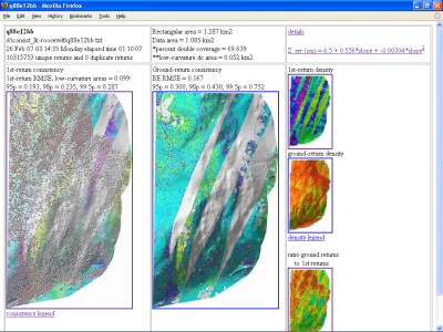 |
CONSISTENCY writes a single HTML page for each analysed tile. This
page
includes medium-scale versions of the 1st-return and ground-return
swath difference images, thumbnails of 1st-return density,
ground-return density, and density-ratio images, summary values for
accuracy and completeness, and links to a difference-curvature-slope
analysis and a text file that summarizes the CONSISTENCY analysis.
Selected elements of this page are discussed here. |
1st-return swath difference
image
|
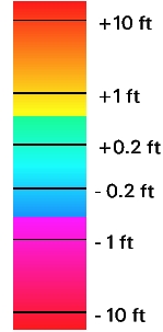
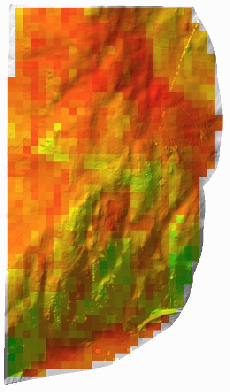
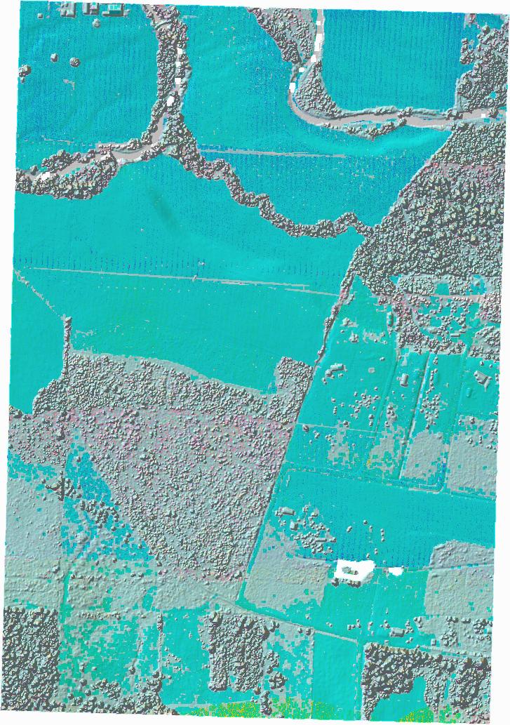
At left is an
example of a 1st-return swath difference image. White areas have no
data. Gray areas (e.g. irregular region at mid- to upper-left) have
data from only a single swath. Colored areas (most of the image) have
data from overlapping swaths; coloring is by the difference between
swaths, following the legend at the right of the image.
Strongly colored (saturated) regions are not strongly
curved and are included in the calculation of RMS Z swath
reproducibility; less strongly colored (unsaturated) regions, such as
the forested area in the lower left quadrant of the image, are strongly
curved, thus prone to large interpolation errors, and are not included
in the calculation of swath reproducibility.
The patterns of differences shown in images like this can
disclose much about how the lidar instrument works and the sources of
error. In particular, this image shows both significant XY displacement
and swath-to-swath tilt, demonstrating that the major source of error
is poor measurement of the orientation of the lidar instrument.
|
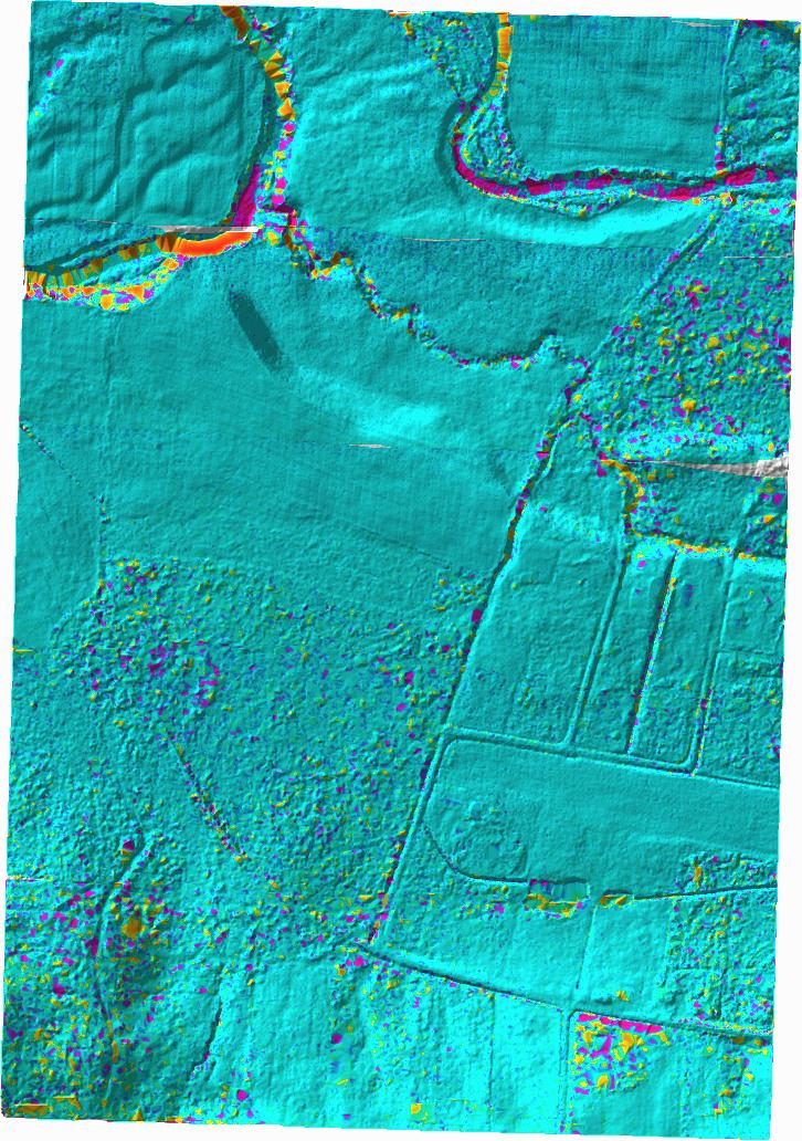
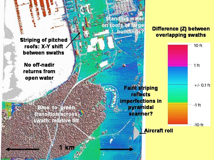
These data were acquired with an instrument that used a
slowly-rotating pyramidal mirror to scan the lidar beam across the
target region. This results in parallel scans of evenly-spaced points
and no pointing error associated with backlash during reversals of
an oscillating mirror. However, it appears that not all faces of the
pyramid have the same orientation with respect to the rotational axis,
causing very minor (cm-level) scan-to-scan errors. Because of the
logarithmic color scale, these are only visible where the
swath-to-swath difference is small.
Some of the largest differences shown in this image are at
the upper left of the image, where a floating marina has risen with the
tide between acquisition of overlapping swaths.
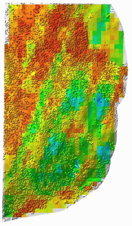
Ground return
swath
difference image
The images above illustrate some of the key features of ground-return
swath difference images. High-curvature areas are not masked. NODATA
masking is less aggressive than for 1st-return swath difference images.
Larger differences in forested areas are common because of a
combination of poor canopy penetration (= larger interpolation errors)
and misclassification of vegetation returns as ground.
Most of the large differences along ravines in the upper part of the
image result from one swath containing ground points at the bottom of
the ravine whereas the overlapping swath lacks ravine-bottom ground
points. The observed accuracy (reproducibility) of the single-swath
DEMs is evidently less than that of the final bare-earth DEM
interpolated from aggregated ground points from all swaths. The
calculated error of the ground model DEM is thus too large because of
overestimated interpolation error. This is counter-balanced, to an
unknown extent, by the failure of the swath-difference calculation to
capture certain long-period and constant errors.
Return-density and
density-ratio images
1st-return
density
|
Ground-return
density
|
 |
Ground-return
density
------------
1st-return
density
|
 |
click for
larger
images |
CONSISTENCY counts the numbers of 1st returns and ground returns in
large
(typically 30 meter or 100 feet) square cells and maps the resulting
point
densities, as well as the ratio # ground returns / # 1st
returns. The resulting images can provide insights into survey
design, lidar instrument sensitivity, and post-processing procedures.
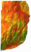
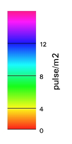
Return-density images are colored by return density, with the central
value at a nominal return density of 2 / (pulse spacing)2.
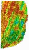
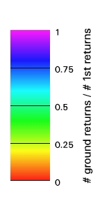
Density-ratio images are colored by ground-return / 1st-return ratio,
with red = 0, blue-green (hue=150) = 0.5, and magenta (hue=300) = 1.
1st-return density and density ratio are shown on a shaded-relief image
of the 1st-return surface. Ground-return density is shown on the
bare-earth surface.
Check the legends
The critical value of abs(dZ) at which difference images jump from
blues and greens to yellows and magentas is an adjustable parameter
within CONSISTENCY. It may change from analysis to analysis. The
point-density color legend will change as known or inferred survey
design changes. Check the legends!
Difference-slope-curvature
graphs
Calculation of P1 and P2 assumes well-mannered distributions of Z
differences, slopes, and curvatures within the analyzed data set.
To facilitate visual exploration of these distributions, CONSISTENCY
constructs a page of graphs of Z difference vs local slope, Z difference vs local curvature, and local
curvature vs local slope for
each analyzed tile, and one for the data set as a whole (except excluded tiles). These pages are
largely self explanatory.
Differences are calculated from rasters derived by bilinear sampling of
TINs constructed from 1st-return data points. Curvature and slope are
calculated from individual swath surfaces using standard ArcInfo
functions with 3x3 kernels. Single-swath curvatures and slopes are
merged to a tile-wide surface; where swaths overlap and there are
multiple calculated curvatures and slopes, the largest curvature or
slope is retained.
Raster cell width is one-half the nominal point spacing. The analyzed
data set includes multiple differences at a single cell where more than
two swaths overlap. Reported N is 1/4 the number of sampled cells.
To minimize storage space, curvatures are rounded to the nearest
multiple of 5 and percent slope values are rounded to the nearest
multiple of 2. Differences are rounded to the nearest cm (difference
<= 1 m), the nearest decimeter (1 m < difference < 2 m), the nearest
meter (2 m < difference <
10 m), or the nearest 5 m.
Prior to calculation of difference-local slope contours and best-fit
lines, the data set is truncated. See P1 & P2,
above.
Text summary pages
(*-l.txt)
For each analyzed tile, CONSISTENCY writes a text
summary page that includes
- analytical results
- attributes of points immediately before and after time gaps that
identify swath breaks, and
- values for a number of adjustable constants within the
CONSISTENCY code.
This text summary page is linked to via details, in the upper right
corner of each individual tile page.
Prerequisites,
assumptions, and simplifications behind the analysis
Tiled data, pulse times available
Consistency analysis presumes that separate, overlapping swaths of
1st-return points can be identified. At the PSLC we have found it
convenient to store individual point-return data in files of all
returns for a given area (tile), with per-return attributes that
include X,Y,Z, and GPS second, GPS week, return number (1, 2, 3, or 4),
and point classification (ground, blunder, unclassified). The first
step in consistency analysis is then to sort the tile on time, separate
into swaths at gaps in the time sequence, and extract 1st returns and
ground returns for each swath.
Comparing swaths
Comparing swaths to observe measurement reproducibility requires
that one observe, or predict, Z values for each swath at the same XY
location. In general, returns in overlapping swaths will not be at
coincident XY locations, so to compare one must predict Z values at
given XY locations for one or both swaths. CONSISTENCY analysis solves
this problem by (1) sampling both swaths at regularly spaced XY
locations (conversion of each swath of point data to a TIN, then
sampling the TIN to a lattice registered to [0,0] ), and (2)
restricting the comparison to regions where interpolation error is
likely to be minimal.
A single swath of lidar data includes returns in a regular X-Y pattern
imposed by the scanning mechanism, with irregularities occasioned by
local relief in the target region and gaps due to non-reflective
targets and (for ground returns) shadowing by forest canopy.
quasi-regular point samples: the raster approximation (why curvature
matters)
Forest canopy is
pathologic
not yet written
Choosing cell sizes
not yet written
No-data masks
not yet written
What is missing?
not yet written
Voids must be found by inspection
Accuracy of return classification is
unquantified
Little leverage on range calibration
Careful survey design can make long-period errors invisible
Spatial correlation of error is not quantified
Users' tolerances for error at different wavelengths have not been
explored
Acknowledgements
Jerry Harless and Diana Martinez (Puget Sound Regional Council),
Phyllis Mann (Kitsap County Department of Emergency Management), Craig
Weaver and Sam Johnson (U.S. Geological Survey), David Harding (NASA),
and numerous partners from city, county, state, tribal and federal
agencies and NGOs, have made the Puget Sound Lidar Consortium work. I
thank them for their effort and the pleasure of working with them.
David Harding, Matthew Boyd (Watershed Sciences), Bob
McGaughey and Steve Reutebuch (US Forest Service), Bill Carter
(University of Florida) and Damir Latypov (TerraPoint) provided
discussion and encouragement regarding the technical content of this
document.