Basic Outline of Setting Up an Ice Sheet in ADINA-F - in general
terms and with a specific example.
Tony Gades, UW Geophysics
Spring 2001
UPDATED LAST: Tuesday, 26 June, 2001 14:01:31
Download this document as
an Adobe Acrobat .pdf file: BasicOutlineofSettingUpanIceSheetinADINA.PDF
The best way to learn some of the idiosyncrasies of ADINA
is to start right in. I personally ended
up wasting quite a bit of time reading through the -very- extensive
documentation. The problem is that
there are endless features to this model that are not of any use to us as ice
modelers - so reading all of that stuff ends up wasting time. The documentation is pretty good though, and
it usually helps you figure out specific answers to specific questions. Another useful feature are the worked
examples.
The instructions I include here are specific to ADINA
V7.4. Earlier versions work differently
and probably later versions will change some things as well. The good thing is that the changes I have
seen in the past year of working with this program have been for the better so
it is worth upgrading and figuring out the differences.
General Overview:
ADINA - (Automatic Dynamic Incremental Nonlinear
Analysis) has several parts to the overall package. The relevant portions of the package to ice flow modeling are:
ADINA-F: for FEM models of fluids
ADINA-T: for doing heat flow
ADINA-PLOT:
for viewing the results of a model.
I start by building a basic ice sheet in ADINA-F. This model will be a basic ice sheet based
on actual Roosevelt Island bed/surface topography. The first goal will be to set up an ice sheet and just let it
flow - without accumulation. Then we
add accumulation and finally heat flow.
A Few General Tips:
1)
As with any program, save often.
2)
The tiny icons in the ADINA gui are not that useful in my
opinion but are redundant with menu options.
I opt for the menu options in describing steps.
3)
There are many ways to do many of the things I describe
here. I have tried many different ways
of doing things and these steps are just what I estimate to be the best or
simplest.
4)
ADINA allows you to create a simple ASCII text script
file of the commands that produce your model (a ".in" file). It seems as though one can get only so far
by using the menu options/icons in the gui and at some stage one must directly
edit the .in file. For example, I could
not determine any other way to specify a velocity function aside from directly
editing the command file. A combination
of using the ADINA-gui and editing the resulting command file seems to be most
efficient.
5)
If you find it simpler to just have a look at a command
script file to figure out how this model works, here is one. RI_IceSheet_NoAccumulation.in
HERE ARE THE STEPS:
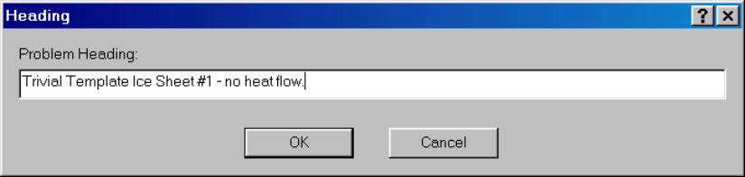
1) Give the model a descriptive title and Save the File:
The heading
is just a label - sort of like a comment at the beginning of some code. In ADINA-F, define a heading by Menu
Option: Control->Heading (this
means click on the Control menu, then select the Heading option)
Save the
file as a ".in" file. This
yields an ASCII text file of all of the commands and allows us to edit the
thing later - this is not the default.
Menu Option: File->SaveAs
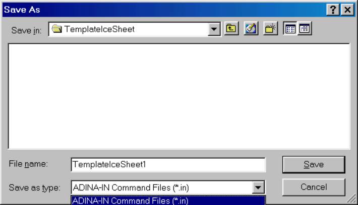
Choose "Save As Type" ADINA-IN Command Files.
2) Decide on a geometry.
a) If complex geometry, then
use the template matlab file to produce a file in ADINA.in format.
b) If simple geometry, then
just make a sketch and make a table of xy or yz points. It is best to label the points clockwise or
counterclockwise around the geometry of the ice sheet.
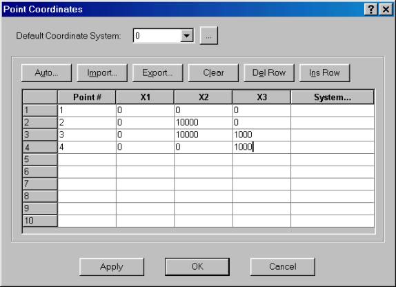
Here is a very simple example in the YZ plane with Z
positive upward, Y positive to the right.
1000 meters thick, flat surface, 10000 meters wide.
Point# X Y Z
1 0 0 0
2 0 10000 0
3 0 10000 1000
4 0 0 1000
Here is how you actually define points from within
ADINA-F. Menu option: Geometry->Points
3) Define the lines that outline the geometry of the ice sheet.
Complex geometries
require using more complex line types.
For example, the "polyline" type allows you to connect (via
linear or other types of interpolation) many points. This is what I use for defining actual ice surfaces and bed.
Very simple ice sheets like the
one above has 2 cliff edges, a surface and a bed requires defining
4 simple lines that are defined only by the 2 end points.
Line# Point1 Point2
1 1 2 (bed)
2 2 3 (RHS
cliff)
3 3 4 (Surface)
4 4 1 (LHS cliff)
In ADINA-F, you define lines from: Geometry->Lines->Define
Click "ADD" button and then fill in the
information:
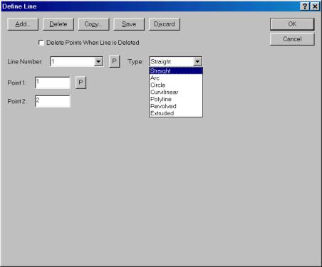
Instead of typing in the points, you can click the
"P" box to the right of the "point 1" entry, this will take
you to the main ADINA screen and then you can just click on the two points that
you wish to use to define line 1. Click
"OK" when done and then "ADD" again and repeat for all 4
lines. There are many line types but
the 2 I find most useful are "straight" and "polyline".
4) Define the 2-D surface or surfaces that define the model.
The
"patch" type surface works well for defining the 2-d surface. Carrying on with the simple ice sheet, one
can define a patch that is bounded by the 4 lines. The "surface" in the 2-D case refers to the body of the
ice sheet.
In ADINA-F Geometry->Surfaces->Define
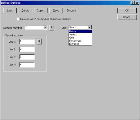
Again, there are many ways to define a surface but a
patch of 4 lines works well.
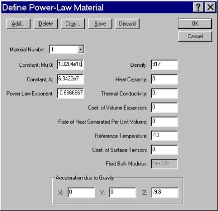
5) Define the Material Model properties
To
read the details of how I got help sorting this out, click on this link: materialmodel.html
Otherwise,
you can just try this for -10C ice:
Menu option: MODEL->MATERIALS->POWER LAW->ADD
Or
you can just try this for -25C ice:
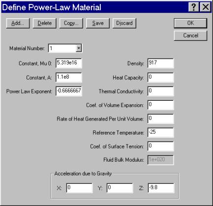
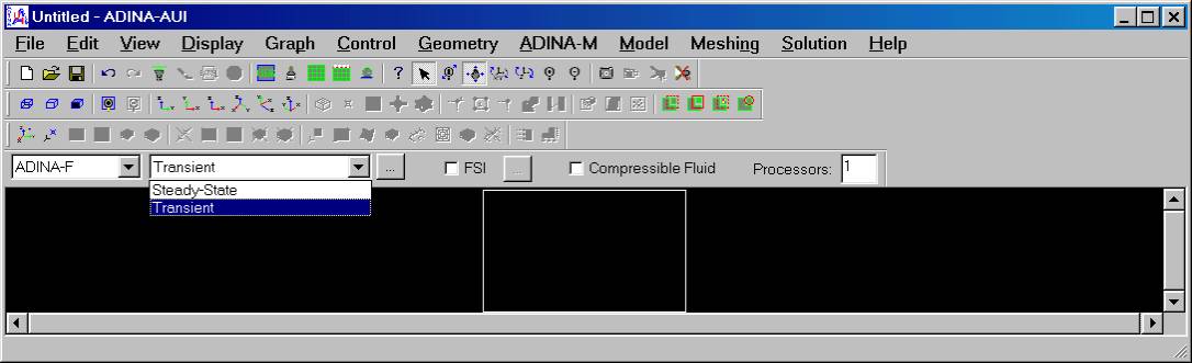
6) Define the flow assumptions; Set solution to transient
Menu Option: MODEL->FLOW
ASSUMPTIONS
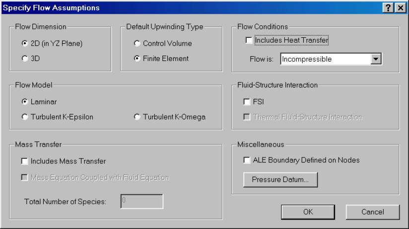
Now click option to
change to transient:
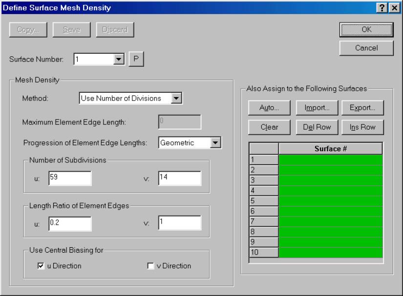
7) Define the mesh density
This is the step where
you define how the mesh nodes are distributed within the model. There are many ways to do this, but this method
allows you to specify that the nodes are preferentially stacked toward the
divide and if desired toward the bottom.
To do this I use the "Geometric" progression of element edge
lengths.
The example below divides
the nodes evenly from top to bottom by:
1) Not selecting the central biasing in v direction.
2) Using a length ratio of 1 in the "v"
direction.
The example
preferentially places nodes toward the horizontal center by:
1) Use central biasing for the u Direction.
2) A value of less than 1 for the "Length ratio
of element edges".
Menu Option: MESHING->MESH
DENSITY->SURFACE
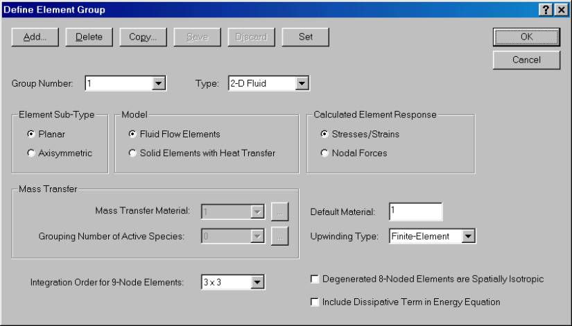
8) Define element type
Menu Option: MESHING->ELEMENT GROUPS->ADD
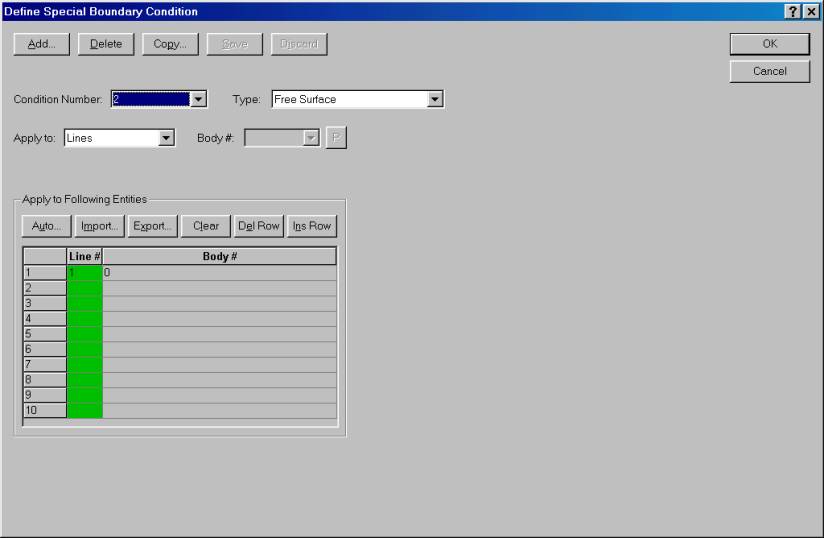
9) Define the boundary conditions for surface and bed
To begin with we want to
have a free surface boundary condition for the ice sheet surface and a no-slip
"wall" condition for the bed.
MENU OPTION: MODEL->SPECIAL
BOUNDARY CONDITIONS->ADD
Add condition 1 for the
wall condition of the bed and apply it to line 3.
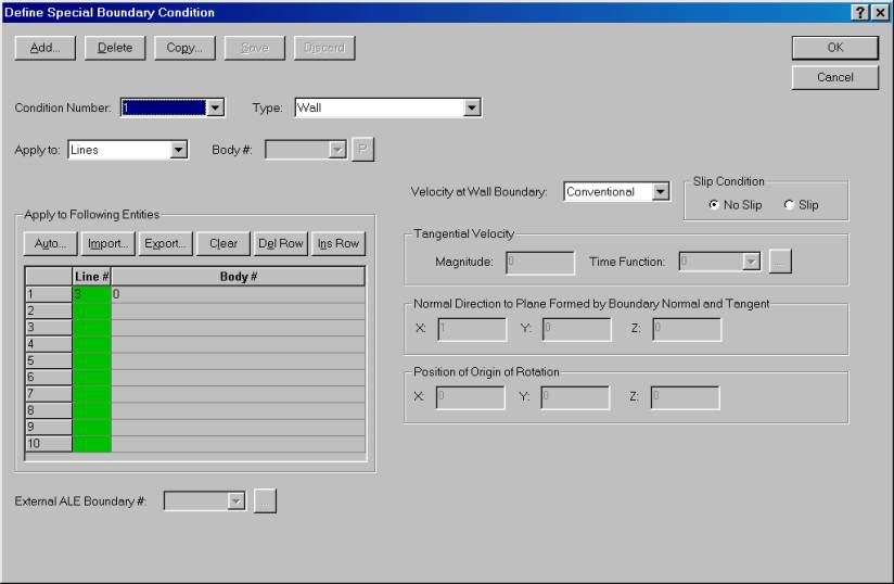
Add condition 2 for the ice
sheet surface and apply it to line 1:
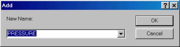
10)Pressure Fixity
For the model to arrive
at a solution, you have to define a pressure zero - this is arbitrary and where
you choose to set the zero doesn't seem to affect the model in any way :
MENU OPTION:
MODEL->USUAL BOUNDARY
CONDITIONS/LOAD->ZERO VALUES->ADD
We need to define a new type of zero value so lets name it PRESSURE.
Then define the
properties of this new zero:
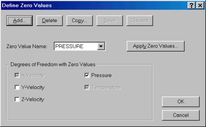
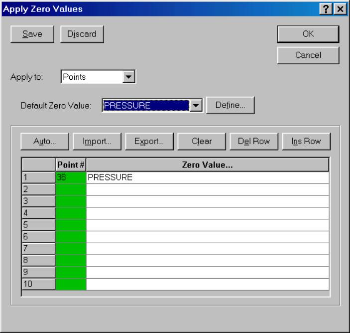
Select only the
"Pressure" box as above, Then click "Apply Zero Values" and apply the zero to some point on the
model - either type in a point number or click in the green box with the mouse
and it will allow you to select a point, hit escape to come back to this
box. Make sure that the zero applied is
the PRESSURE zero that we just defined as shown below.
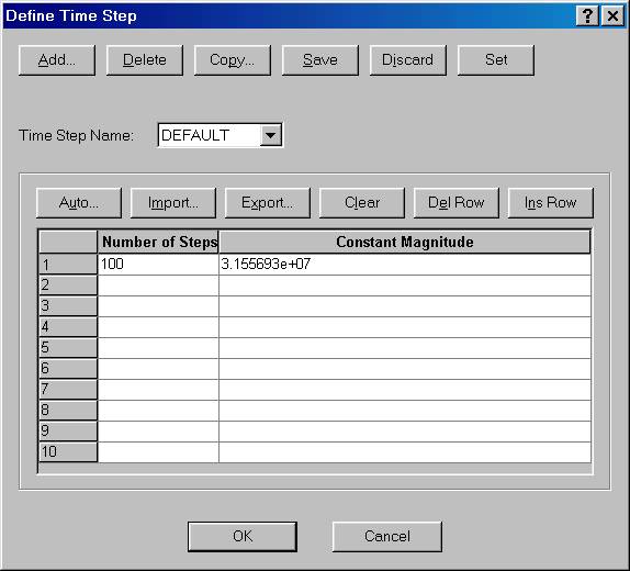
11) Define Time steps
I set this entire model
up in MKS units. This means time is in
seconds.
1 year = 3.155693e+07 seconds
So, that is the magnitude
needed for a single year time step. To start,
set up the model for 100 steps of 1year each.
MENU OPTION: CONTROL->TIME
STEP
12) Add equilibrium velocity conditions at margin. (INCOMPLETE)
In this next and final step, we have to prescribe a
velocity profile at the margins of the ice sheet that give equilibrium assuming
some accumulation rate. That is, a
velocity profile that gets rid of an amount of ice equal to sum total added at
the surface. Paterson, Chapter 11,
details all of this.
The logistics of adding this velocity profile are much
easier to do if you actually edit the command file - I don't know of any better
way to do this.
The general idea is that first you specify a
"line-function" as a table of values and then you apply a
"velocity load" to a line in your model. The table can include as many values as desired - the more
values, the higher resolution the function you specify. This method is a bit clunky but appears to
be the only option.
So, if I want to specify a velocity function like this
for example:
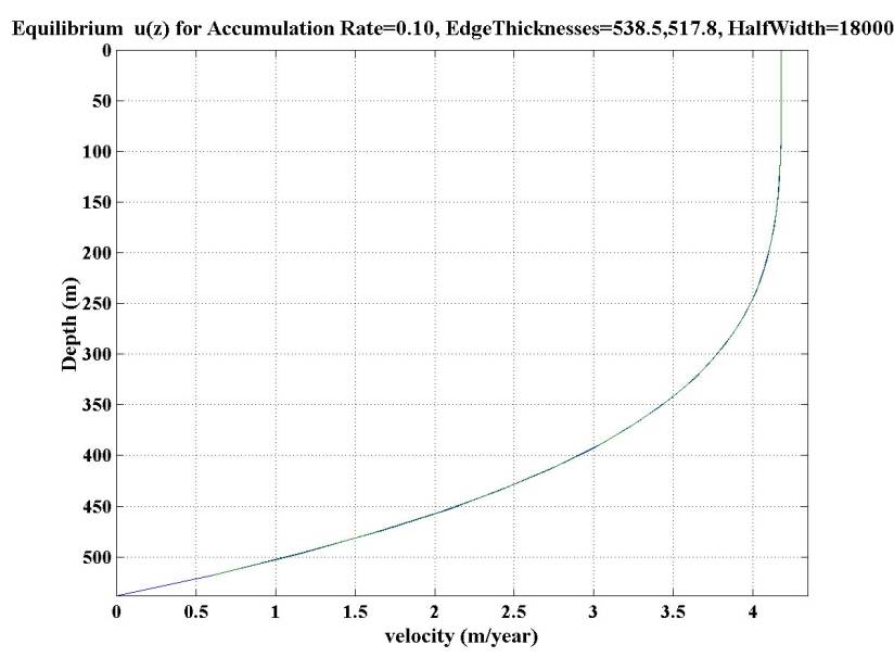
I would do it by
specifying a table like this (in this case I arbitrarily have chosen a table
length of 26 points):
Again, units are MKS so
meters/second - an unfortunate set of units for ice flow...
*
* Ice Stream Edge Velocity Profile for equilibrium given
* Equilibrium
u(z) for Accumulation Rate=0.10, EdgeThicknesses=538.5,517.8,
HalfWidth=18000.0
*
LINE-FUNCTIO NAME=1 TYPE=TABULAR NPOINT=26
@CLEAR
1 1.324922e-007
2 1.324918e-007
3 1.324867e-007
4 1.324647e-007
5 1.324053e-007
6 1.322802e-007
7 1.320526e-007
8 1.316778e-007
9 1.311029e-007
10 1.302668e-007
11 1.291004e-007
12 1.275262e-007
13 1.254589e-007
14 1.228048e-007
15 1.194622e-007
16 1.153212e-007
17 1.102637e-007
18 1.041635e-007
19 9.688641e-008
20 8.828990e-008
21 7.822338e-008
22 6.652811e-008
23 5.303723e-008
24 3.757571e-008
25 1.996040e-008
26 1.126558e-022
@
*
LOAD VELOCITY NAME=1 VX=FREE VY=-1.00000000000000 VZ=FREE
*
* Velocity Profile for equilibrium given
* Equilibrium
u(z) for Accumulation Rate=0.10, EdgeThicknesses=538.5,517.8, HalfWidth=18000.0
*
LINE-FUNCTIO NAME=2 TYPE=TABULAR NPOINT=26
@CLEAR
1 1.922721e-008
2 3.629097e-008
3 5.134995e-008
4 6.456770e-008
5 7.610079e-008
6 8.609884e-008
7 9.470451e-008
8 1.020535e-007
9 1.082746e-007
10 1.134895e-007
11 1.178130e-007
12 1.213531e-007
13 1.242107e-007
14 1.264796e-007
15 1.282469e-007
16 1.295926e-007
17 1.305898e-007
18 1.313045e-007
19 1.317960e-007
20 1.321164e-007
21 1.323109e-007
22 1.324179e-007
23 1.324687e-007
24 1.324875e-007
25 1.324919e-007
26 1.324922e-007
@
*
LOAD VELOCITY NAME=2 VX=FREE VY=1.00000000000000 VZ=FREE
*
Here is an example where these velocities are actually
applied. RI_IceSheet_NoAccumulation.in
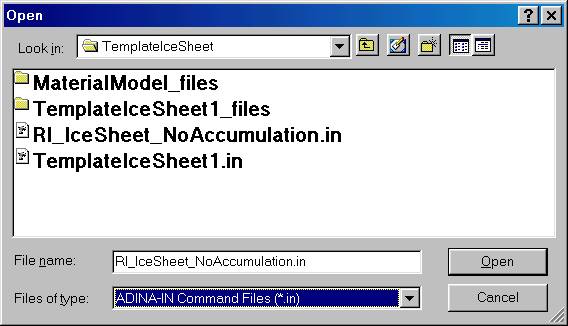
13) TRY IT
To give it a try, start up
ADINA-AUI and load this file: RI_IceSheet_NoAccumulation.in
Start up ADINA, then Menu Option: FILE->OPEN
make sure to change file type to "ADINA-IN Command
Files" as below.
Then do a load plot to
see the model setup. This is
accomplished by clicking on the icon shown in this image:
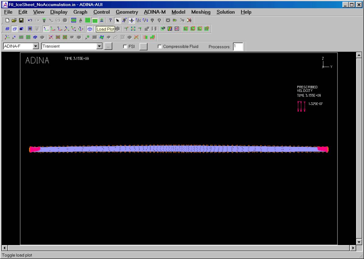
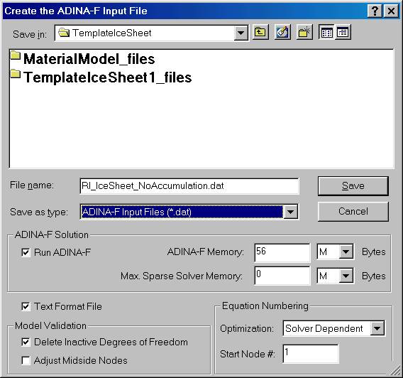
Now run the thing. Menu Option: SOLUTION->DATA FILE/RUN
You have to give the
output ".dat" file a name.
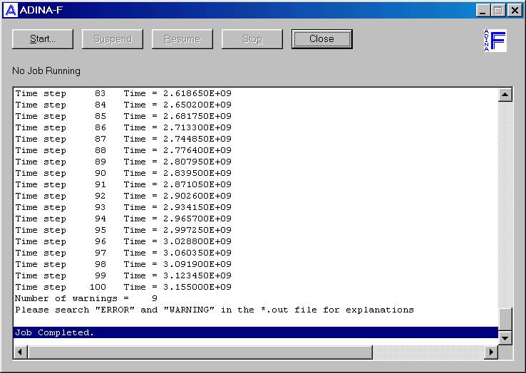
The initial time steps
will bring up some warnings - this is the result of the model not being stable
with the initial setup. This settles
out after a few time steps.
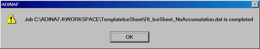
Eventually you should get
this popup box:
14) EXAMINE THE RESULTS
We have to switch
programs to ADINA-PLOT.
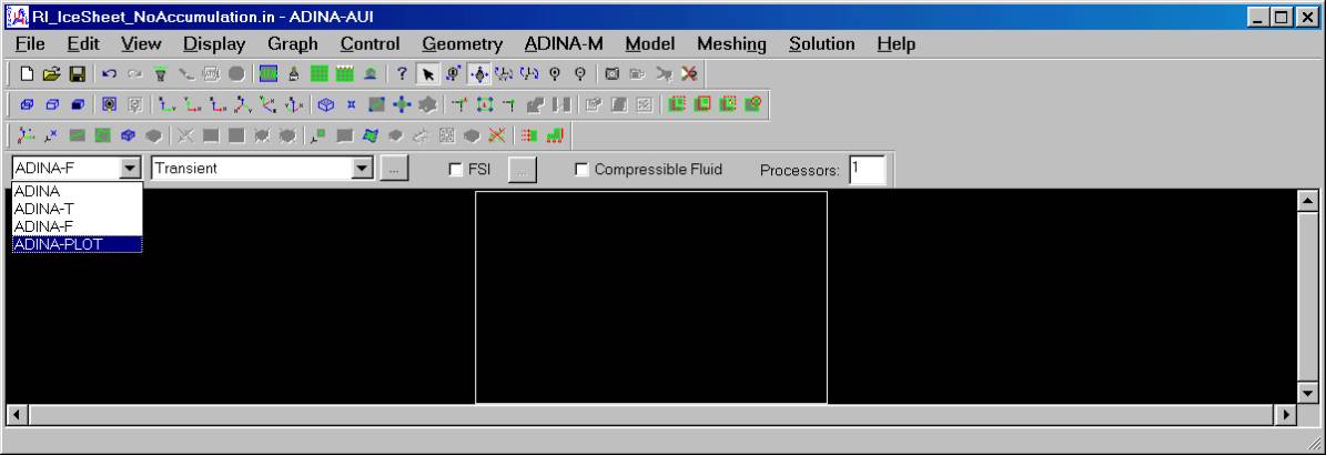
Click yes to the
question:
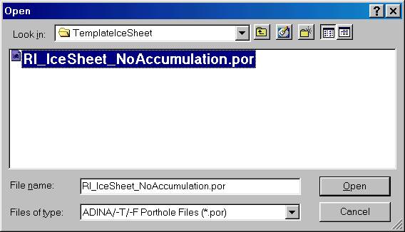
Now we need to load the
results file.
Menu Option: FILE->OPEN
and select the porthole
(results) file we generated by running the model.
It is good to do a mesh
plot which shows the results and the deformed mesh:
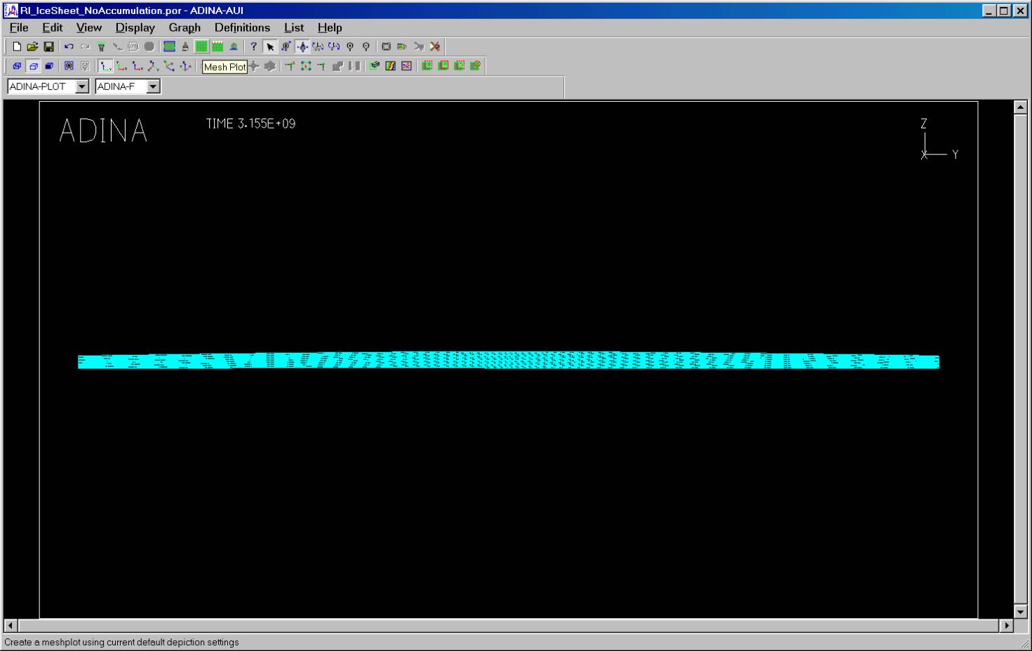
But, the best way to view
the results is to get rid of the mesh.
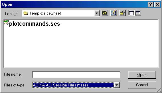
There is a standard set of settings that I make to the plotting
options. I have included in this
file: plotcommands.ses
This file sets up the
plotting preferences to only plot the outline of the model. Load this sequence of commands with MENU
OPTION: FILE->OPEN then select file type of
"Session Files" and load the
plotcommands.ses file. The
commands will automatically run.
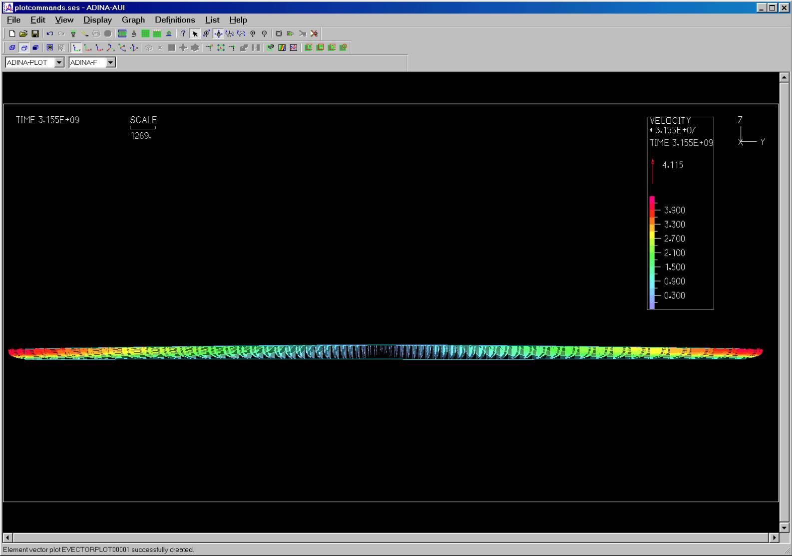
This will yield an image something
like this - a vector plot showing the end velocity field. In the plotcommands file, I have selected
that the velocity vectors be scaled to yield meters/year rather than the
useless meters/second.
After the