Local Basis Function | J Michael Brown

A focus on the other 99.9% of Earth

This page contains information about fitting (thermodynamic) data. Actually - the issue is how to represent arbitrary behavior of measurements when theory does not provide adequate guidance. This is a particular problem for fluids and aqueous solutions at high pressure. Publications are filled with arbitrary representations that are typically "global" (any model parameter has influence on model predictions everywhere) and these models frequently use custom choices for polynomial (and non-polynomial) terms. Here an alternative approach is advocated. "local basis functions" are required to fit data (within uncertainty) while providing satisfactory behavior for interpolation or extrapolation. Being "local" means that parameters for an equation of state can be modified in one regime of pressure and temperature without impacting an excellent representation in another regime. see: Brown, J.M., (2018) Local basis function representations of thermodynamic surfaces: Water at high pressure and temperature as an example, Fluid Phase Equilibria, 463C, 18-31, doi.org/10.1016/j.fluid.2018.02.001

Key ideas:

Local basis function (LBF) representations of any surface (with 1, 2, 3, or more independent variables) can have arbitrarily small misfit (specified in their construction).
Derivatives of the LBF can also be fit to data and/or made to be smooth or have appropriate asymptotic behavior.
Energies (Gibbs, Helmholz, etc) can be represented with LBF and all thermodynamic properties can be accurately predicted.
LBF representations for equations of state are easily modified to better match measurements
LBF formulations are orders of magnitude faster in execution than common forms of equations of state

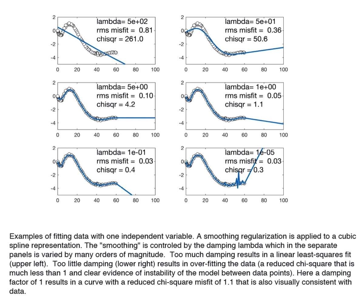
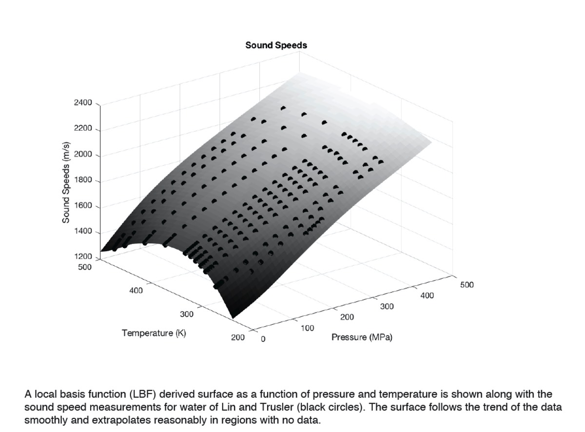
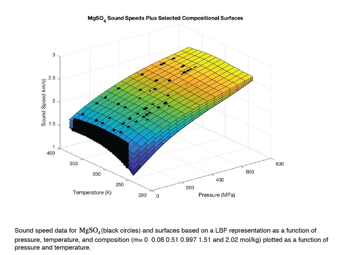
Examples on the right show local basis function (LBF) fits to data with one, two, or three independent variables (pressure, temperature, composition). These examples are given in tutorial MATLAB live scripts that are linked below. Three items are downloadable.: (1) a paper describing the tools and methods (2) a set of toolbox functions, (3) a set of examples.

Basic tools provided in the toolbox include:

a general LBF data fitter,
a function that converts measured sound speeds (as a function of pressure and temperature) into high pressure densities, specific heats, and Gibbs energy (based on a predict and correct algorithm to integrate sound speeds),
a function to convert thermodynamic results (densities, specific heats, and Gibbs energies) into a LBF Gibbs energy representation, and
a function to analytically calculate thermodynamic properties from a Gibbs energy LBF representation. The background image on this page is a example of properties predicted from such a representation for water.

Link to the manuscript
Link to published reprint
Link to the toolbox
Link to the example scripts

If you just want to see a pdf version of the examples try these links:
1. fitting data
2. Converting sound speeds into equations of state LBF representations
3. modification of the EOS for water under high pressure conditions

Required: MATLAB 2016 or later (capable of running "live scripts" and the curve fitting toolbox. Preview versions of MATLAB and the curve fitting toolbox (free use for 30 days) can be obtained from mathworks.com.